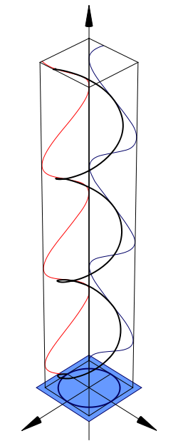
ОписаниеPolarisation (Circular).svg	The direction of the helix relative to the central axis represents the direction of the electric field of the circularly polarized light at each point in space. The blue and red lines are projections of the helix onto two planes at right angles. There is an version which is identical to this original with the exception of phase indictors to make the phase relationship of its components clearer. Refer to Other Versions section below.
Дата	12/02/07
Источник	Own drawing down in Mathematica, edited in the open source program Inscape.  Это векторное изображение было создано с помощью Inkscape .
Автор	inductiveload
Права (Повторное использование этого файла)	Public domainPublic domainfalsefalse Я, владелец авторских прав на это произведение, передаю его в общественное достояние. Это разрешение действует по всему миру. В некоторых странах это не может быть возможно юридически, в таком случае: Я даю право кому угодно использовать данное произведение в любых целях без каких-либо условий, за исключением таких условий, которые требуются по закону.
Другие версии	Производные работы от этого файла:  Polarisation (Circular) With Phase Indicators.svg Linear polarisation Elliptical polarisation

This figure requires the use of Arrow3D, which is not included in the StandardPackages (as of Feb 2007). This can be obtained from Wolfram Research at this location. The required packages are:

<< Graphics`
<< Arrow3D`Arrow3D`

The code is:

wavefunction = ParametricPlot3D[{Sin[4t], -Cos[4t], t}, {t, 0, 5}, 
BoxRatios -> {1, 1, 4}, ImageSize -> 400, Boxed -> False, Axes -> 
    False, PlotPoints -> 600, ViewPoint -> {2, 2, 2}, PlotRange -> All]

repsi = ParametricPlot3D[{Sin[4t], -1, t, RGBColor[1, 0, 0]}, {t, 0, 5}, 
    BoxRatios -> {4, 1, 1}, ImageSize -> 500,
     Boxed -> False, Axes -> False, PlotPoints -> 600, PlotRange -> All]

impsi = ParametricPlot3D[{-1, -Cos[4t], t, RGBColor[0, 0, 102/255]}, {t, 0, \
5}, BoxRatios -> {4, 1, 1}, ImageSize -> 500, Boxed -> False, Axes -> False, 
      PlotPoints -> 600, PlotRange -> All]

end = ParametricPlot3D[{Sin[t], -Cos[t], 0}, {t, 0, 
    2π}, BoxRatios -> {4, 1, 1}, ImageSize -> 500, Boxed -> False, 
    Axes -> False, PlotPoints -> 600, PlotRange -> All]

xaxis = Graphics3D[Arrow3D[{0, 0, -1}, {0, 
  0, 6}, HeadSize -> UniformSize[.5], HeadColor -> Black]]

uaxis = Graphics3D[Arrow3D[{0, -1, 0}, {0, 3, 0}, HeadSize -> 
    UniformSize[.5], HeadColor -> Black]]

vaxis = Graphics3D[Arrow3D[{-1, 0, 0}, {3, 0, 0}, HeadSize -> 
    UniformSize[.5], HeadColor -> Black]]

plane = Graphics3D[Polygon[{{1.2, 1.2, 0}, {1.2, -1.2,
   0}, {-1.2, -1.2, 0}, {-1.2, 1.2, 0}}]]

crate = WireFrame[Graphics3D[Cuboid[{1, 1, 0}, {-1, -1, 5}]]]

Show[wavefunction, xaxis, uaxis, vaxis, plane, repsi, impsi, end, crate]